Note
Go to the end to download the full example code.
Spatially heterogeneous atmbc (Weil et al)#
Weill, S., et al. « Coupling Water Flow and Solute Transport into a Physically-Based Surface–Subsurface Hydrological Model ». Advances in Water Resources, vol. 34, no 1, janvier 2011, p. 128‑36. DOI.org (Crossref), https://doi.org/10.1016/j.advwatres.2010.10.001.
This example shows how to use pyCATHY object to create spatially and temporally variable atmbc conditions
Estimated time to run the notebook = 5min
# !! run preprocessor change the DEM shape !
# dtm_13 does not have the same shape anymore!

import os

import matplotlib.pyplot as plt
import numpy as np
import pandas as pd

import pyCATHY.meshtools as mt
from pyCATHY import cathy_tools
from pyCATHY.importers import cathy_inputs as in_CT
from pyCATHY.importers import cathy_outputs as out_CT
from pyCATHY.plotters import cathy_plots as cplt
path2prj = "../SSHydro/"  # add your local path here
simu = cathy_tools.CATHY(dirName=path2prj,
                         prj_name="atmbc_spatially_from_weill"
                         )

simu.create_mesh_vtk(verbose=True)
🏁 Initiate CATHY object
🍳 gfortran compilation
👟 Run preprocessor

 wbb...

 searching the dtm_13.val input file...
 assigned nodata value =  -9999.0000000000000

 number of processed cells =         400

 ...wbb completed

 rn...
 csort I...
 ...completed

 depit...
 dem modifications =            0
 dem modifications =            0 (total)
 ...completed

 csort II...
 ...completed

 cca...

 contour curvature threshold value =    9.99999996E+11
 ...completed

 smean...
 mean (min,max) facet slope =  0.052056253 ( 0.020000000, 0.053851648)
 ...completed

 dsf...
 the drainage direction of the outlet cell (           8 ) is used
 ...completed

 hg...
 ...completed

 saving the data in the basin_b/basin_i files...

 ...rn completed

 mrbb...


 Select the header type:
 0) None
 1) ESRI ascii file
 2) GRASS ascii file
 (Ctrl C to exit)

 ->
 Select the nodata value:
 (Ctrl C to exit)

 ->
 Select the pointer system:
 1) HAP system
 2) Arc/Gis system
 (Ctrl C to exit)

 ->  ~~~~~~~~~~~~~~~~~~~~~~~~~~~~~~~~~~~~~~~~~~

 dem file

 min value = 0.335000E+00
 max value = 0.100000E+01
 number of cells =   400
 mean value = 0.667500E+00

 writing the output file...

 ~~~~~~~~~~~~~~~~~~~~~~~~~~~~~~~~~~~~~~~~~~

 lakes_map file

 min value =     0
 max value =     0
 number of cells =   400
 mean value =     0.000000

 writing the output file...

 ~~~~~~~~~~~~~~~~~~~~~~~~~~~~~~~~~~~~~~~~~~

 zone file

 min value =     1
 max value =     1
 number of cells =   400
 mean value =     1.000000

 writing the output file...

 ~~~~~~~~~~~~~~~~~~~~~~~~~~~~~~~~~~~~~~~~~~

 dtm_w_1 file

 min value = 0.515524E+00
 max value = 0.100000E+01
 number of cells =   400
 mean value = 0.607575E+00

 writing the output file...

 ~~~~~~~~~~~~~~~~~~~~~~~~~~~~~~~~~~~~~~~~~~

 dtm_w_2 file

 min value = 0.000000E+00
 max value = 0.484476E+00
 number of cells =   400
 mean value = 0.392425E+00

 writing the output file...

 ~~~~~~~~~~~~~~~~~~~~~~~~~~~~~~~~~~~~~~~~~~

 dtm_p_outflow_1 file

 min value =     4
 max value =     8
 number of cells =   400
 mean value =     4.200000

 writing the output file...

 ~~~~~~~~~~~~~~~~~~~~~~~~~~~~~~~~~~~~~~~~~~

 dtm_p_outflow_2 file

 min value =     0
 max value =     9
 number of cells =   400
 mean value =     6.792500

 writing the output file...

 ~~~~~~~~~~~~~~~~~~~~~~~~~~~~~~~~~~~~~~~~~~

 A_inflow file

 min value = 0.000000000000E+00
 max value = 0.997499787031E+02
 number of cells =   400
 mean value = 0.388447785378E+01

 writing the output file...

 ~~~~~~~~~~~~~~~~~~~~~~~~~~~~~~~~~~~~~~~~~~

 dtm_local_slope_1 file

 min value = 0.200000E-01
 max value = 0.500000E-01
 number of cells =   400
 mean value = 0.485000E-01

 writing the output file...

 ~~~~~~~~~~~~~~~~~~~~~~~~~~~~~~~~~~~~~~~~~~

 dtm_local_slope_2 file

 min value = 0.000000E+00
 max value = 0.494975E-01
 number of cells =   400
 mean value = 0.400930E-01

 writing the output file...

 ~~~~~~~~~~~~~~~~~~~~~~~~~~~~~~~~~~~~~~~~~~

 dtm_epl_1 file

 min value = 0.500000E+00
 max value = 0.500000E+00
 number of cells =   400
 mean value = 0.500000E+00

 writing the output file...

 ~~~~~~~~~~~~~~~~~~~~~~~~~~~~~~~~~~~~~~~~~~

 dtm_epl_2 file

 min value = 0.000000E+00
 max value = 0.707107E+00
 number of cells =   400
 mean value = 0.572757E+00

 writing the output file...

 ~~~~~~~~~~~~~~~~~~~~~~~~~~~~~~~~~~~~~~~~~~

 dtm_kSs1_sf_1 file

 min value = 0.240040E+02
 max value = 0.240040E+02
 number of cells =   400
 mean value = 0.240040E+02

 writing the output file...

 ~~~~~~~~~~~~~~~~~~~~~~~~~~~~~~~~~~~~~~~~~~

 dtm_kSs1_sf_2 file

 min value = 0.000000E+00
 max value = 0.240040E+02
 number of cells =   400
 mean value = 0.194432E+02

 writing the output file...

 ~~~~~~~~~~~~~~~~~~~~~~~~~~~~~~~~~~~~~~~~~~

 dtm_Ws1_sf file

 min value = 0.100000E+01
 max value = 0.100000E+01
 number of cells =   400
 mean value = 0.100000E+01

 writing the output file...

 ~~~~~~~~~~~~~~~~~~~~~~~~~~~~~~~~~~~~~~~~~~

 dtm_Ws1_sf_2 file

 min value = 0.000000E+00
 max value = 0.100000E+01
 number of cells =   400
 mean value = 0.810000E+00

 writing the output file...

 ~~~~~~~~~~~~~~~~~~~~~~~~~~~~~~~~~~~~~~~~~~

 dtm_b1_sf file

 min value = 0.000000E+00
 max value = 0.000000E+00
 number of cells =   400
 mean value = 0.000000E+00

 writing the output file...

 ~~~~~~~~~~~~~~~~~~~~~~~~~~~~~~~~~~~~~~~~~~

 dtm_y1_sf file

 min value = 0.000000E+00
 max value = 0.000000E+00
 number of cells =   400
 mean value = 0.000000E+00

 writing the output file...

 ~~~~~~~~~~~~~~~~~~~~~~~~~~~~~~~~~~~~~~~~~~

 dtm_hcID file

 min value =     0
 max value =     0
 number of cells =   400
 mean value =     0.000000

 writing the output file...

 ~~~~~~~~~~~~~~~~~~~~~~~~~~~~~~~~~~~~~~~~~~

 dtm_q_output file

 min value =     0
 max value =     0
 number of cells =   400
 mean value =     0.000000

 writing the output file...

 ~~~~~~~~~~~~~~~~~~~~~~~~~~~~~~~~~~~~~~~~~~

 dtm_nrc file

 min value = 0.100000E+01
 max value = 0.100000E+01
 number of cells =   400
 mean value = 0.100000E+01

 writing the output file...

 ...mrbb completed

 bb2shp...

 writing file river_net.shp

Note: The following floating-point exceptions are signalling: IEEE_UNDERFLOW_FLAG IEEE_DENORMAL

🔄 Update parm file
🔄 Update hap.in file
🔄 Update dem_parameters file
🔄 Update dem_parameters file
🛠  Recompile src files [4s]
🍳 gfortran compilation [10s]
✅ Compilation successful!
👟 Run processor
b'\n\n IPRT1=3: Program terminating after output of X, Y, Z coordinate values\n'
grid3d = simu.read_outputs('grid3d')

# np.shape(simu.DEM)

# DEM, dem_header = simu.read_inputs('dem')
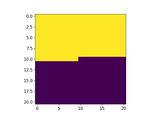
t_atmbc = [0,86400]
v_atmbc = np.zeros(int(grid3d['nnod']))
v_atmbc[0:int(len(np.zeros(int(grid3d['nnod'])))/2)] = 1e-7

v_atmbc_mat = np.reshape(v_atmbc,[np.shape(simu.DEM)[0]+1,
                                  np.shape(simu.DEM)[1]+1
                                  ])
fig, ax = plt.subplots()
ax.imshow(v_atmbc_mat)

# np.shape([v_atmbc]*len(t_atmbc))

simu.update_atmbc(
                    HSPATM=0,
                    IETO=0,
                    time=t_atmbc,
                    netValue=[v_atmbc]*len(t_atmbc)
                  )
🔄 Update atmbc
🔄 Update parm file
simu.run_processor(IPRT1=2,
                    DTMIN=1e-2,
                    DTMAX=1e2,
                    DELTAT=5,
                   TRAFLAG=0,
                   verbose=False
                   )

# cplt.show_spatial_atmbc()
🔄 Update parm file
🛠  Recompile src files [10s]
🍳 gfortran compilation [16s]
✅ Compilation successful!
👟 Run processor
cplt.show_vtk(
    unit="pressure",
    timeStep=1,
    notebook=False,
    path=simu.workdir + simu.project_name + "/vtk/",
    savefig=True,
)
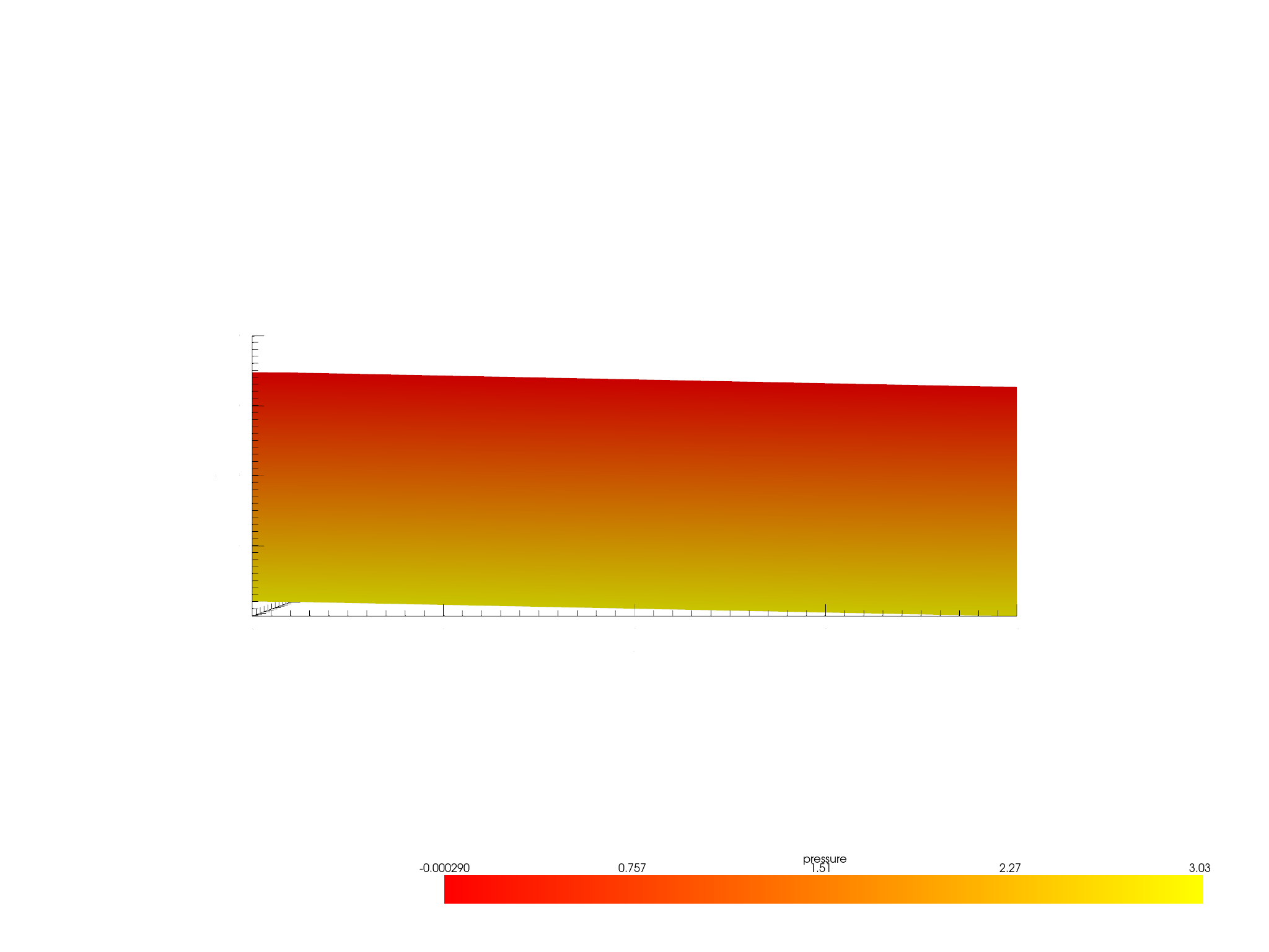
plot pressure
figure saved/home/z0272571a@campus.csic.es/Nextcloud/BenCSIC/Codes/BenjMy/pycathy_wrapper/examples/SSHydro/../SSHydro/atmbc_spatially_from_weill/vtk/101.vtkpressure.png
cplt.show_vtk_TL(
                unit="pressure",
                notebook=False,
                path=simu.workdir + simu.project_name + "/vtk/",
                show=False,
                x_units='days',
                clim = [0.55,0.70],
                savefig=True,
            )
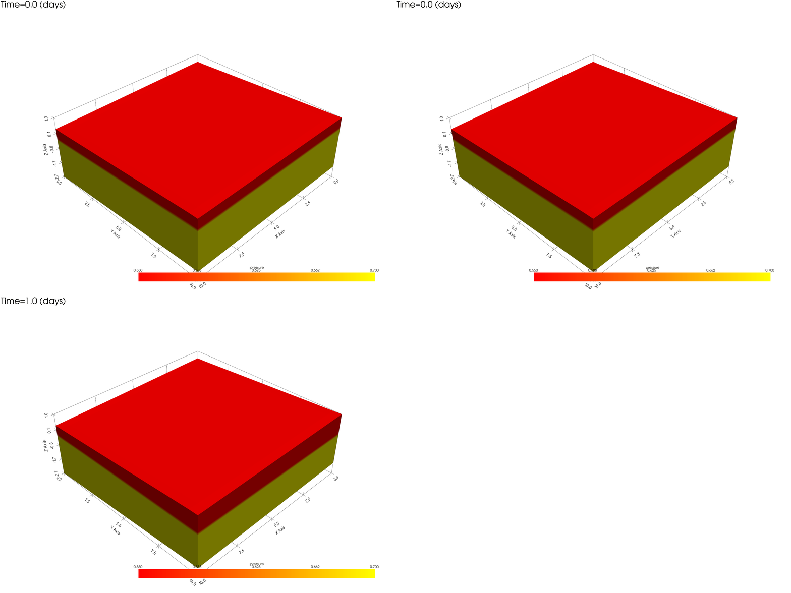
days
plot pressure
Time= [0.]
/home/z0272571a@campus.csic.es/Nextcloud/BenCSIC/Codes/BenjMy/pycathy_wrapper/examples/SSHydro/../SSHydro/atmbc_spatially_from_weill/vtk/100.vtk
[0.]
/home/z0272571a@campus.csic.es/Nextcloud/BenCSIC/Codes/BenjMy/pycathy_wrapper/examples/SSHydro/../SSHydro/atmbc_spatially_from_weill/vtk/101.vtk
[0.01953]
/home/z0272571a@campus.csic.es/Nextcloud/BenCSIC/Codes/BenjMy/pycathy_wrapper/examples/SSHydro/../SSHydro/atmbc_spatially_from_weill/vtk/102.vtk
[86400.]
/home/z0272571a@campus.csic.es/Nextcloud/BenCSIC/Codes/BenjMy/pycathy_wrapper/examples/SSHydro/../SSHydro/atmbc_spatially_from_weill/vtk/103.vtk
[86400.]
gif saved/home/z0272571a@campus.csic.es/Nextcloud/BenCSIC/Codes/BenjMy/pycathy_wrapper/examples/SSHydro/../SSHydro/atmbc_spatially_from_weill/vtk/pressure.gif
Total running time of the script: (0 minutes 33.132 seconds)