Output plots part 2

Weill, S., et al. « Coupling Water Flow and Solute Transport into a Physically-Based Surface–Subsurface Hydrological Model ». Advances in Water Resources, vol. 34, no 1, janvier 2011, p. 128‑36. DOI.org (Crossref), https://doi.org/10.1016/j.advwatres.2010.10.001.

This example shows how to use pyCATHY object to plot the most common ouputs of the hydrological model.

Estimated time to run the notebook = 5min

Here we need to import cathy_tools class that control the CATHY core files preprocessing and processing We also import cathy_plots to render the results

from pyCATHY import cathy_tools
from pyCATHY.plotters import cathy_plots as cplt

if you add True to verbose, the processor log will be printed in the window shell

path2prj = "../SSHydro/"  # add your local path here
simu = cathy_tools.CATHY(dirName=path2prj,
                    prj_name="weil_exemple_outputs_plot"
                    )

simu.run_preprocessor()

🏁 Initiate CATHY object
🍳 gfortran compilation
👟 Run preprocessor

simu.read_inputs('atmbc')
# simu.create_mesh_bounds_df(
#     'nansfdirbc',
#     simu.grid3d["mesh3d_nodes"],
#     t_atmbc,
# )

# print(simu.mesh_bound_cond_df.head())
# print("BC columns:", list(simu.mesh_bound_cond_df.columns))

# Apply no-flow to all lateral/bottom boundaries
simu.update_nansfneubc(no_flow=True)
simu.update_nansfdirbc(no_flow=True)
simu.update_sfbc(no_flow=True)

shortcut set_BC_laterals mesh dataframe
🔄 Update parm file
🔄 Update hap.in file
🔄 Update dem_parameters file
🔄 Update dem_parameters file
🔄 Update parm file

simu.run_processor(IPRT1=2,
                    DTMIN=1e-2,
                    DTMAX=1e2,
                    DELTAT=5,
                   TRAFLAG=0,
                   verbose=False
                   )

🔄 Update parm file
🛠  Recompile src files [5s]
🍳 gfortran compilation [13s]
✅ Compilation successful!
👟 Run processor

simu.show(prop="hgsfdet")

simu.show(prop="dtcoupling", yprop="Atmpot-d")

/home/runner/work/pycathy_wrapper/pycathy_wrapper/pyCATHY/importers/cathy_outputs.py:385: UserWarning: Input line 3 contained no data and will not be counted towards `max_rows=236`.  This differs from the behaviour in NumPy <=1.22 which counted lines rather than rows.  If desired, the previous behaviour can be achieved by using `itertools.islice`.
Please see the 1.23 release notes for an example on how to do this.  If you wish to ignore this warning, use `warnings.filterwarnings`.  This warning is expected to be removed in the future and is given only once per `loadtxt` call.
  dtcoupling = np.loadtxt(dtcoupling_file, skiprows=2, max_rows=2 + nstep)

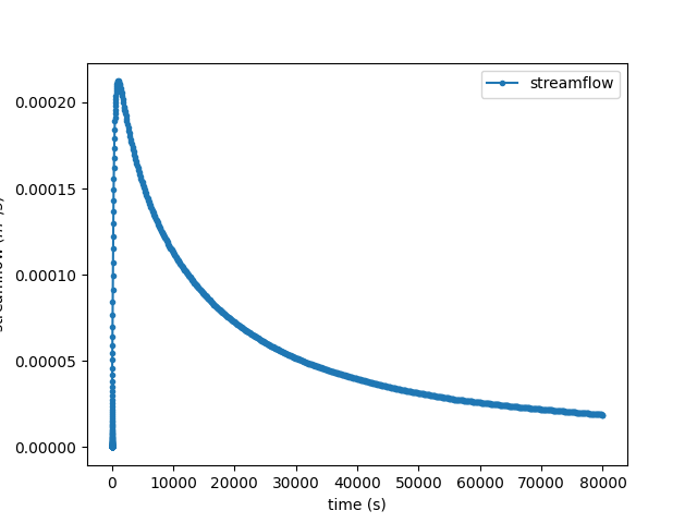
simu.show(prop="hgraph")

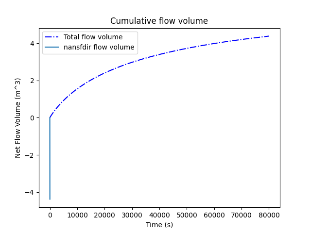
simu.show(prop="cumflowvol")

To select another time step change the value in the function argument

cplt.show_vtk(
    unit="pressure",
    timeStep=1,
    notebook=False,
    path=simu.workdir + "/weil_exemple_outputs_plot/vtk/",
)

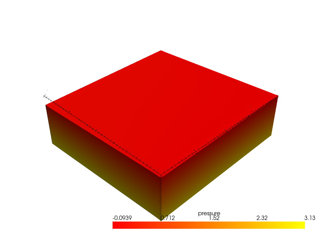
plot pressure

cplt.show_vtk(

unit=”saturation”, timeStep=1, notebook=False, path=simu.workdir + “/my_cathy_prj/vtk/”,

)

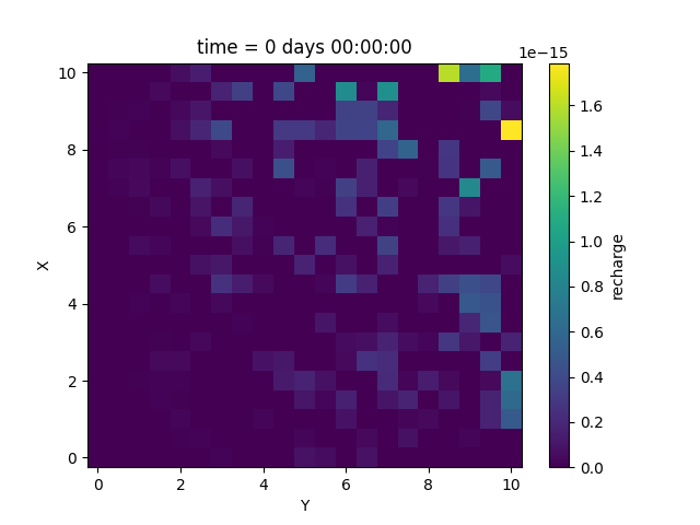
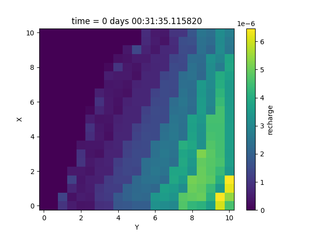
df_recharge = simu.read_outputs('recharge')
xr_recharge = df_recharge.set_index(['time','X','Y']).to_xarray()

import matplotlib.pyplot as plt

fig, ax = plt.subplots()
xr_recharge['recharge'].isel(time=0).plot.imshow(ax=ax)


fig, ax = plt.subplots()
xr_recharge['recharge'].isel(time=1).plot.imshow(ax=ax)

• 
• 

<matplotlib.image.AxesImage object at 0x7fae36f6bf70>