Output plots part 1

Weill, S., et al. « Coupling Water Flow and Solute Transport into a Physically-Based Surface–Subsurface Hydrological Model ». Advances in Water Resources, vol. 34, no 1, janvier 2011, p. 128‑36. DOI.org (Crossref), https://doi.org/10.1016/j.advwatres.2010.10.001.

This example shows how to use pyCATHY object to plot the most common ouputs of the hydrological model.

Estimated time to run the notebook = 5min

Here we need to import cathy_tools class that control the CATHY core files preprocessing and processing We also import cathy_plots to render the results

from pyCATHY import cathy_tools
from pyCATHY.plotters import cathy_plots as cplt
import pyvista as pv
import os
import matplotlib.pyplot as plt

if you add True to verbose, the processor log will be printed in the window shell

path2prj = "weil_exemple_outputs_plot1"  # add your local path here
simu = cathy_tools.CATHY(dirName=path2prj)
simu.run_preprocessor()
simu.run_processor(IPRT1=2,
                    DTMIN=1e-2,
                    DTMAX=1e2,
                    DELTAT=5,
                    TRAFLAG=0,
                    verbose=False
                    )

🏁 Initiate CATHY object
🍳 gfortran compilation
👟 Run preprocessor
🔄 Update parm file
🔄 Update hap.in file
🔄 Update dem_parameters file
🔄 Update dem_parameters file
🛠  Recompile src files [5s]
🍳 gfortran compilation [11s]
b''
👟 Run processor

df_sw, _ = simu.read_outputs('sw')
df_sw.head()

	0	1	2	3	4	5	6	7	8	9	10	11	12	13	14	15	16	17	18	19	20	21	22	23	24	25	26	27	28	29	30	31	32	33	34	35	36	37	38	39	...	7016	7017	7018	7019	7020	7021	7022	7023	7024	7025	7026	7027	7028	7029	7030	7031	7032	7033	7034	7035	7036	7037	7038	7039	7040	7041	7042	7043	7044	7045	7046	7047	7048	7049	7050	7051	7052	7053	7054	7055
Time
0.00000	1.000000	1.000000	1.000000	1.000000	1.000000	1.000000	1.000000	1.000000	1.000000	1.000000	1.000000	1.000000	1.000000	1.000000	1.000000	1.000000	1.000000	1.000000	1.000000	1.000000	1.000000	1.000000	1.000000	1.000000	1.000000	1.000000	1.000000	1.000000	1.000000	1.000000	1.000000	1.000000	1.000000	1.000000	1.000000	1.000000	1.000000	1.000000	1.000000	1.000000	...	1.0	1.0	1.0	1.0	1.0	1.0	1.0	1.0	1.0	1.0	1.0	1.0	1.0	1.0	1.0	1.0	1.0	1.0	1.0	1.0	1.0	1.0	1.0	1.0	1.0	1.0	1.0	1.0	1.0	1.0	1.0	1.0	1.0	1.0	1.0	1.0	1.0	1.0	1.0	1.0
1895.11582	0.686681	0.688439	0.689260	0.689816	0.690354	0.690762	0.691186	0.691529	0.691910	0.692281	0.692698	0.693121	0.693597	0.694194	0.694924	0.695890	0.697219	0.699154	0.701742	0.708113	0.710240	0.690039	0.690454	0.692535	0.692936	0.693486	0.693991	0.694504	0.694993	0.695479	0.695949	0.696475	0.697041	0.697722	0.698518	0.699569	0.700933	0.702768	0.705330	0.709040	...	1.0	1.0	1.0	1.0	1.0	1.0	1.0	1.0	1.0	1.0	1.0	1.0	1.0	1.0	1.0	1.0	1.0	1.0	1.0	1.0	1.0	1.0	1.0	1.0	1.0	1.0	1.0	1.0	1.0	1.0	1.0	1.0	1.0	1.0	1.0	1.0	1.0	1.0	1.0	1.0
3666.91023	0.655817	0.657207	0.657718	0.658108	0.658493	0.658816	0.659167	0.659469	0.659805	0.660141	0.660514	0.660899	0.661331	0.661849	0.662468	0.663246	0.664281	0.665721	0.667496	0.672289	0.673416	0.658255	0.658917	0.660504	0.660679	0.661049	0.661392	0.661745	0.662091	0.662448	0.662803	0.663199	0.663633	0.664152	0.664765	0.665558	0.666576	0.667943	0.669838	0.672429	...	1.0	1.0	1.0	1.0	1.0	1.0	1.0	1.0	1.0	1.0	1.0	1.0	1.0	1.0	1.0	1.0	1.0	1.0	1.0	1.0	1.0	1.0	1.0	1.0	1.0	1.0	1.0	1.0	1.0	1.0	1.0	1.0	1.0	1.0	1.0	1.0	1.0	1.0	1.0	1.0
7266.91023	0.626298	0.627181	0.627431	0.627604	0.627765	0.627907	0.628082	0.628229	0.628418	0.628599	0.628833	0.629081	0.629383	0.629768	0.630255	0.630890	0.631756	0.632959	0.634299	0.638162	0.638892	0.627849	0.628339	0.629545	0.629491	0.629659	0.629821	0.630007	0.630190	0.630404	0.630632	0.630904	0.631223	0.631619	0.632116	0.632758	0.633594	0.634705	0.636205	0.638076	...	1.0	1.0	1.0	1.0	1.0	1.0	1.0	1.0	1.0	1.0	1.0	1.0	1.0	1.0	1.0	1.0	1.0	1.0	1.0	1.0	1.0	1.0	1.0	1.0	1.0	1.0	1.0	1.0	1.0	1.0	1.0	1.0	1.0	1.0	1.0	1.0	1.0	1.0	1.0	1.0
10866.91020	0.609930	0.610632	0.610809	0.610921	0.611022	0.611111	0.611229	0.611324	0.611452	0.611569	0.611729	0.611895	0.612101	0.612367	0.612711	0.613168	0.613799	0.614689	0.615580	0.618658	0.619467	0.611197	0.611591	0.612642	0.612516	0.612611	0.612698	0.612805	0.612906	0.613033	0.613171	0.613344	0.613556	0.613830	0.614189	0.614665	0.615294	0.616137	0.617280	0.618644	...	1.0	1.0	1.0	1.0	1.0	1.0	1.0	1.0	1.0	1.0	1.0	1.0	1.0	1.0	1.0	1.0	1.0	1.0	1.0	1.0	1.0	1.0	1.0	1.0	1.0	1.0	1.0	1.0	1.0	1.0	1.0	1.0	1.0	1.0	1.0	1.0	1.0	1.0	1.0	1.0

5 rows × 7056 columns

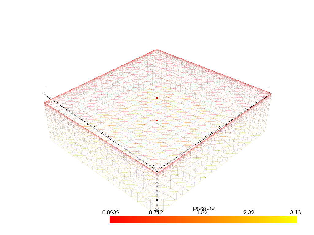
node, node_pos = simu.find_nearest_node([5,5,-1])
node2, node_pos2 = simu.find_nearest_node([5,5,1])
print(node_pos[0])

[ 5.      5.     -1.0725]

pl = pv.Plotter(notebook=False)
cplt.show_vtk(unit="pressure",
              timeStep=1,
              path=os.path.join(simu.workdir,
                                simu.project_name,
                                'vtk'
                                ),
              style='wireframe',
              opacity=0.1,
              ax=pl,
              )
pl.add_points(node_pos[0],
              color='red'
              )
pl.add_points(node_pos2[0],
              color='red'
              )
pl.show()

plot pressure

fig, ax = plt.subplots()
df_sw[node].plot(ax=ax)
df_sw[node2].plot(ax=ax)
ax.set_xlabel('time (s)')
ax.set_ylabel('saturation (-)')

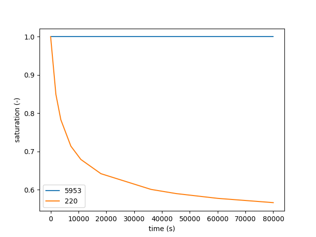
Text(42.722222222222214, 0.5, 'saturation (-)')

df_psi = simu.read_outputs('psi')
# df_psi.head()
fig, ax = plt.subplots()
ax.plot(df_psi.index, df_psi.iloc[:,node[0]])
ax.plot(df_psi.index, df_psi.iloc[:,node2[0]])
ax.set_xlabel('time (s)')
ax.set_ylabel('pressure head (m)')

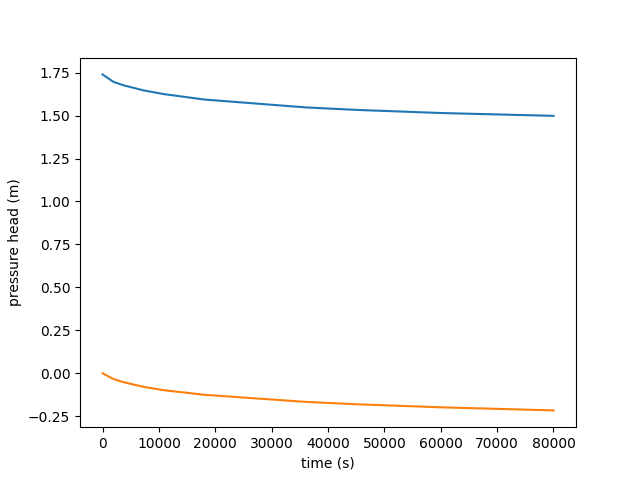
Text(22.472222222222214, 0.5, 'pressure head (m)')