Update with spatially and temporally distributed atmospheric boundary conditions (bc)

This tutorial demonstrates how to update atmospheric boundary conditions (bc) using spatially and temporally distributed data in a hydrological model.

Reference: Weill, S., et al. « Coupling Water Flow and Solute Transport into a Physically-Based Surface–Subsurface Hydrological Model ». Advances in Water Resources, vol. 34, no 1, janvier 2011, p. 128‑36. DOI.org (Crossref), https://doi.org/10.1016/j.advwatres.2010.10.001.

This example uses the pyCATHY wrapper for the CATHY model to reproduce results from the Weill et al. dataset. The notebook is interactive and can be executed in sections to observe the intermediate results. It can also be shared for collaborative work without any installation required.

Estimated time to run the notebook = 5 minutes

# Import necessary libraries
import os
import matplotlib.pyplot as plt
import numpy as np
import pandas as pd
import pyvista as pv

# Import pyCATHY modules for handling mesh, inputs, and outputs
import pyCATHY.meshtools as mt
from pyCATHY import cathy_tools
from pyCATHY.importers import cathy_inputs as in_CT
from pyCATHY.importers import cathy_outputs as out_CT
from pyCATHY.plotters import cathy_plots as cplt

Define the project directory and model name. This example uses ‘atmbc_spatially_from_weill’.

path2prj = "../SSHydro/"  # Replace with your local project path
simu = cathy_tools.CATHY(dirName=path2prj, prj_name="atmbc_spatially_from_weill_withnodata")
figpath = "../results/DA_ET_test/"  # Path to store figures/results

🏁 Initiate CATHY object

Read the DEM input file

DEM, dem_header = simu.read_inputs('dem')

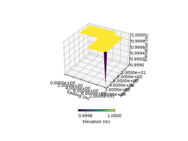
# Create a new DEM array filled with ones and add irregular boundary and invalid values (-9999)
DEM_new = np.ones(np.shape(DEM))  # Initialize new DEM with ones
DEM_new[-1, -1] = 1 - 1e-3  # Adjust a specific corner value
DEM_new[10:20, 0:10] = -9999  # Add an interior block of invalid values to simulate an irregular boundary
DEM_new[0:3, 15:20] = -9999  # Add an interior block of invalid values to simulate an irregular boundary

# Update the CATHY inputs with the modified DEM
simu.update_prepo_inputs(DEM_new)

# Visualize the updated DEM
simu.show_input('dem')

Traceback (most recent call last):
  File "/home/runner/work/pycathy_wrapper/pycathy_wrapper/examples/SSHydro/plot_3d_spatial_atmbc_from_weill.py", line 51, in <module>
    simu.update_prepo_inputs(DEM_new)
  File "/home/runner/work/pycathy_wrapper/pycathy_wrapper/pyCATHY/cathy_tools.py", line 1217, in update_prepo_inputs
    self.update_zone()
  File "/home/runner/work/pycathy_wrapper/pycathy_wrapper/pyCATHY/cathy_tools.py", line 1696, in update_zone
    self.update_parm()
  File "/home/runner/work/pycathy_wrapper/pycathy_wrapper/pyCATHY/cathy_tools.py", line 1858, in update_parm
    self.update_cathyH(
  File "/home/runner/work/pycathy_wrapper/pycathy_wrapper/pyCATHY/cathy_tools.py", line 776, in update_cathyH
    self.update_veg_map()
  File "/home/runner/work/pycathy_wrapper/pycathy_wrapper/pyCATHY/cathy_tools.py", line 3353, in update_veg_map
    indice_veg, str_hd_rootmap = in_CT.read_root_map(os.path.join(
  File "/home/runner/work/pycathy_wrapper/pycathy_wrapper/pyCATHY/importers/cathy_inputs.py", line 529, in read_root_map
    with open(os.path.join(rootmapfile), "r") as f:  # open the file for reading
FileNotFoundError: [Errno 2] No such file or directory: '/home/runner/work/pycathy_wrapper/pycathy_wrapper/examples/SSHydro/../SSHydro/atmbc_spatially_from_weill_withnodata/input/veg_map'

Run the preprocessor to handle inputs and generate the mesh

simu.run_preprocessor()

# Create a 3D mesh visualization (VTK format)
simu.create_mesh_vtk(verbose=True)

# Load the 3D grid output
grid3d = simu.read_outputs('grid3d')

# Set parameters for elevation
simu.dem_parameters
elevation_increment = 0.5 / 21  # Define elevation increment per row
elevation_matrix = np.ones([21, 21])  # Initialize the elevation matrix

# Populate elevation_matrix with incremental values based on row index
for row in range(21):
    elevation_matrix[row, :] += row * elevation_increment

# Set up time intervals and cycles for the boundary condition
interval = 5  # Number of intervals
ncycles = 7   # Number of cycles
t_atmbc = np.linspace(1e-3, 36e3 * ncycles, interval * ncycles)  # Time vector

# Atmospheric boundary condition value
v_atmbc_value = -2e-7  # Set the boundary condition value

# Check if the number of nodes matches the flattened elevation matrix
if int(grid3d['nnod']) == len(np.ravel(elevation_matrix)):
    # Calculate the atmospheric boundary condition for each node based on elevation
    v_atmbc = np.ones(int(grid3d['nnod'])) * v_atmbc_value * np.ravel(elevation_matrix)
else:
    # For cases where the number of nodes doesn't match, calculate for all nodes
    v_atmbc_all_nodes = np.ones(len(np.ravel(elevation_matrix))) * v_atmbc_value * np.ravel(np.exp(elevation_matrix**2))

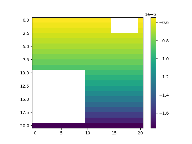
    # Reshape the boundary condition values to match the DEM shape
    v_atmbc_mat = np.reshape(v_atmbc_all_nodes, [np.shape(simu.DEM)[0] + 1, np.shape(simu.DEM)[0] + 1])

    # Mask invalid values in the DEM (-9999) by setting them to NaN
    maskDEM_novalid = np.where(DEM_new == -9999)
    v_atmbc_mat[maskDEM_novalid] = np.nan

    # Flatten the masked matrix and remove NaN values
    v_atmbc = np.ravel(v_atmbc_mat)
    v_atmbc = v_atmbc[~np.isnan(v_atmbc)]  # Use ~np.isnan to filter out NaN values

# Visualize the spatial variation of the atmospheric boundary condition
fig, ax = plt.subplots()
img = ax.imshow(v_atmbc_mat)
plt.colorbar(img)

# Update the atmospheric boundary condition (ATMB) parameters in CATHY
simu.update_atmbc(
    HSPATM=0,
    IETO=0,
    time=t_atmbc,
    netValue=[v_atmbc] * len(t_atmbc)  # Apply the same boundary condition at all times
)

# Update the model parameters (time control) in CATHY
simu.update_parm(TIMPRTi=t_atmbc)

# Run the model processor with specified parameters for time stepping and output control
simu.run_processor(
    IPRT1=2,  # Print results at time step 2
    DTMIN=1e-2,  # Minimum time step
    DTMAX=1e2,  # Maximum time step
    DELTAT=5,  # Time increment
    TRAFLAG=0,  # Transport flag off
    VTKF=2,  # Output VTK format
    verbose=True  # Turn off verbose mode
)

# Visualize the atmospheric boundary conditions in space using vtk
cplt.show_vtk(
    unit="pressure",
    timeStep=1,  # Time step to display
    notebook=False,
    path=simu.workdir + "/atmbc_spatially_from_weill/vtk/",  # Path to VTK files
    savefig=True,  # Save the figure
)

# Create a time-lapse visualization of pressure distribution over time
# cplt.show_vtk_TL(
#     unit="saturation",
#     notebook=False,
#     path=simu.workdir + simu.project_name + "/vtk/",  # Path to VTK files
#     show=False,  # Disable showing the plot
#     x_units='days',  # Time units
#     clim=[0.55, 0.70],  # Color limits for pressure values
#     savefig=True,  # Save the figure
# )